Typical usage Scenarios and Examples

Choose a task from the list below. For more details on alternative options, follow the links to the individual tools being used.

Note that by default it is assumed that ICC profile have the file extension .icm, but that on Apple OS X and Unix/Linux platforms, the .icc extension is expected and should be used.

Profiling Displays

    Checking you can access your display

    Adjusting and Calibrating a displays

    Adjusting, calibrating and profiling in one step

    Creating display test values

    Taking readings from a display

    Creating a display profile

    Installing a display profile

    Expert tips when measuring displays

    Calibrating and profiling a display that doesn't have VideoLUT access.


Profiling Scanners and other input devices such as cameras

    Types of test charts

    Taking readings from a scanner

    Creating a scanner profile


Profiling Printers

    Creating a print profile test chart

    Printing a print profile test chart

    Reading a print test chart using an instrument

    Reading a print test chart using a scanner

    Creating a printer profile

    Choosing a black generation curve


Calibrating Printers

    Calibrated print workflows

    Creating a print calibration test chart

    Creating a printer calibration

    Using a printer calibration

    How profile ink limits are handled when calibration is being used


Linking Profiles


Transforming colorspaces of raster files


Profiling Displays

Argyll supports adjusting, calibrating and profiling of displays using one of a number of instruments - see instruments for a current list.  Adjustment and calibration are prior steps to profiling, in which the display is adjusted using it's screen controls,  and then per channel lookup tables are created to make it meet a well behaved response of the desired type. The  process following that of creating a display profile is then similar to that of all other output devices :- first a set of device colorspace test values needs to be created to exercise the display, then these values need to be displayed, while taking measurements of the resulting colors using the instrument. Finally, the device value/measured color values need to be converted into an ICC profile.

Checking you can access your display

You might first want to check that you are accessing and can calibrate your display. You can do this using the dispwin tool. If you just run dispwin it will create a test window and run through a series of test colors before checking that the VideoLUT can be accessed by the display. If you invoke the usage for dispwin (by giving it an unrecognized option, e.g. -?) then it will show a list of available displays next to the -d flag. Make sure that you are accessing the display you intend to calibrate and profile, and that the VideoLUT is effective (the -r flag can be used to just run the VideoLUT test). You can also try clearing the VideoLUTs using the -c flag, and loading a deliberately strange looking calibration strange.cal that is provided in the Argyll ref directory.

Note that calibrating and/or profiling remote displays is possible using X11 or a web browser (see -d option of dispcal and dispread), or by using some external program to send test colors to a display (see -C and -M options of dispcal and dispread), but you may want to refer to Calibrating and profiling a display that doesn't have VideoLUT access.

Adjusting and Calibrating Displays

Please read What's the difference between Calibration and Characterization ? if you are unclear as to the difference .

The first step is to decide what the target should be for adjustment and calibration. This boils down to three things: The desired brightness, the desired white point, and the desired response curve. The native brightness and white points of a display may be different to the desired characteristics for some purposes. For instance, for graphic arts use, it might be desirable to run with a warmer white point of about 5000 degrees Kelvin, rather than the default display white point of 6500 to 9000 Kelvin. Some LCD displays are too bright to compare to printed material under available lighting, so it might be desirable to reduce the maximum brightness.

You can run dispcal -r to check on how your display is currently set up. (you may have to run this as dispcal -yl -r for an LCD display, or dispcal -yc -r for a CRT display with most of the colorimeter instruments. If so, this will apply to all of the following examples.)

Once this is done, dispcal can be run to guide you through the display adjustments, and then calibrate it. By default, the brightness and white point will be kept the same as the devices natural brightness and white point. The default response curve is a gamma of 2.4, except for Apple OS X systems prior to 10.6 where a gamma of 1.8 is the default. 2.4 is close to that of  many monitors, and close to that of the sRGB colorspace.

A typical calibration that leaves the brightness and white point alone, might be:

dispcal -v TargetA

which will result in a "TargetA.cal" calibration file, that can then be used during the profiling stage.

If the absolutely native response of the display is desired during profiling, then calibration should be skipped, and the linear.cal file from the "ref" directory used instead as the argument to the -k flag of dispread.

Dispcal will display a test window in the middle of the screen, and issue a series of instructions about placing the instrument on the display. You may need to make sure that the display cursor is not in the test window, and it may also be necessary to disable any screensaver and powersavers before starting the process, although both dispcal and dispread will attempt to do this for you. It's also highly desirable on CRT's, to clear your screen of any white or bright background images or windows (running your shell window with white text on a black background helps a lot here.), or at least keep any bright areas away from the test window, and be careful not to change anything on the display while the readings are taken. Lots of bright images or windows can affect the ability to measure the black point accurately, and changing images on the display can cause inconsistency in the readings,  and leading to poor results. LCD displays seem to be less influenced by what else is on the screen.

If dispcal is run without arguments, it will provide a usage screen. The -c parameter allows selecting a communication port for an instrument, or selecting the instrument you want to use,  and the -d option allows selecting a target display on a multi-display system. On some multi-monitor systems, it may not be possible to independently calibrate and profile each display if they appear as one single screen to the operating system, or if it is not possible to set separate video lookup tables for each display. You can change the position and size of the test window using the -P parameter. You can determine how best to arrange the test window, as well as whether each display has separate video lookup capability, by experimenting with the dispwin tool.

For a more detailed discussion on interactively adjusting the display controls using dispcal, see dispcal-adjustment. Once you have adjusted and calibrated your display, you can move on to the next step.

When you have calibrated and profiled your display, you can keep it calibrated using the dispcal -u option.

Adjusting, calibrating and profiling in one step.

If a simple matrix/shaper display profile is all that is desired, dispcal can be used to do this, permitting display adjustment, calibration and profiling all in one operation. This is done by using the dispcal -o flag:

dispcal -v -o TargetA

This will create both a TargetA.cal file, but also a TargetA.icm file. See -o and -O for other variations.

For more flexibility in creating a display profile, the separate steps of creating characterization test values using targen, reading them from the display using dispread, and then creating a profile using colprof are used. The following steps illustrate this:

Profiling in several steps: Creating display test values

If the dispcal has not been used to create a display profile at the same time as adjustment and calibration, then it can be used to create a suitable set of calibration curves as the first step, or the calibration step can be omitted, and the display cansimply be profiled.

The first step in profiling any output device, is to create a set of device colorspace test values. The important parameters needed are:
For a display device,  the colorspace will be RGB. The number of test patches will depend somewhat on what quality profile you want to make, what type of profile you want to make, and how long you are prepared to wait when testing the display.
At a minimum, a few hundred values are needed. A matrix/shaper type of profile can get by with fewer test values, while a LUT based profile will give better results if more test values are used. A typical number might be 200-600 or so values, while 1000-2000 is not an unreasonable number for a high quality characterization of a display.

To assist the choice of test patch values, it can help to have a rough idea of how the device behaves. This could be in the form of an ICC profile of a similar device, or a lower quality, or previous profile for that particular device. If one were going to make a very high quality LUT based profile, then it might be worthwhile to make up a smaller, preliminary shaper/matrix profile using a few hundred test points, before embarking on testing the device with several thousand.

Lets say that we ultimately want to make a profile for the device "DisplayA", the simplest approach is to make a set of test values that is independent of the characteristics of the particular device:

targen -v  -d3 -f500 DisplayA

If there is a preliminary or previous profile called "OldDisplay" available, and we want to try creating a "pre-conditioned" set of test values that will more efficiently sample the device response, then the following would achieve this:

targen -v  -d3 -f500 -cOldDisplay.icm DisplayA

The output of targen will be the file DisplayA.ti1, containing the device space test values, as well as expected CIE values used for chart recognition purposes.

Profiling in several steps: Taking readings from a display

First it is necessary to connect your measurement instrument to your computer, and check which communication port it is connected to. In the following example, it is assumed that the instrument is connected to the default port 1, which is either the first USB instrument found, or serial port found. Invoking dispread so as to display the usage information (by using a flag -? or --) will list the identified serial and USB ports, and their labels.

dispread -v DisplayA

If we created a calibration for the display using dispcal, then we will want to use this when we take the display readings (e.g. TargetA.cal from the calibration example)..

dispread -v -k TargetA.cal DisplayA

dispread will display a test window in the middle of the screen, and issue a series of instructions about placing the instrument on the display. You may need to make sure that the display cursor is not in the test window, and it may also be necessary to disable any screensaver before starting the process. Exactly the same facilities are provided to select alternate displays using the -d parameter, and an alternate location and size for the test window using the -P parameter as with dispcal.

Profiling in several steps: Creating a display profile

There are two basic choices of profile type for a display, a shaper/matrix profile, or a LUT based profile. They have different tradeoffs. A shaper/matrix profile will work well on a well behaved display, that is one that behaves in an additive color manner, will give very smooth looking results, and needs fewer test points to create. A LUT based profile on the other hand, will model any display behaviour more accurately, and can accommodate gamut mapping and different intent tables. Often it can show some unevenness and contouring in the results though.

To create a matrix/shaper profile, the following suffices:

colprof -v -D"Display A" -qm -as DisplayA

For a LUT based profile, where gamut mapping is desired, then a source profile will need to be provided to define the source gamut. For instance, if the display profile was likely to be linked to a CMYK printing source profile, say "swop.icm" or "fogra39l.icm", then the following would suffice:

colprof -v -D"Display A" -qm -S fogra39l.icm -cpp -dmt DisplayA

Make sure you check the delta E report at the end of the profile creation, to see if the profile is behaving reasonably.
If a calibration file was used with dispread, then it will be converted to a vcgt tag in the profile, so that the operating system or other system color tools load the lookup curves into the display hardware, when the profile is used.

Installing a display profile

dispwin provides a convenient way of installing a profile as the default system profile for the chosen display:

dispwin -I DisplayA.icm

This also sets the display to the calibration contained in the profile. If you want to try out a calibration before installing the profile, using dispwin without the -I option will load a calibration (ICC profile or .cal file) into the current display.

Some systems will automatically set the display to the calibration contained in the installed profile (ie. OS X), while on other systems (ie. MSWindows and Linux/X11) it is necessary to use some tool to do this. On MSWindows XP you could install the optional  Microsoft Color Control Panel Applet for Windows XP available for download from Microsoft to do this, but NOTE however that it seems to have a bug, in that it sometimes associates the profiles with the wrong monitor entry. Other display calibration tools will often install a similar tool, so beware of there being multiple, competing programs. [ Commonly these will be in your Start->Programs->Startup folder. ]
On Microsoft Vista, you need to use dispwin -L or some other tool to load the installed profiles calibration at startup.

To use dispwin to load the installed profiles calibration to the display, use

dispwin -L

As per usual, you can select the appropriate display using the -d flag.

This can be automated on MSWindows and X11/Linux by adding this command to an appropriate startup script.
More system specific details, including how to create such startup scripts are here.

If you are using Microsoft Vista, there is a known bug in Vista that resets the calibration every time a fade-in effect is executed, which happens if you lock and unlock the computer, resume from sleep or hibernate, or User Access Control is activated. Using dispwin -L may not restore the calibration, because Vista filters out setting (what it thinks) is a calibration that is already loaded. Use dispwin -c -L as a workaround, as this will first clear the calibration, then re-load the current calibration.

On X11/Linux systems, you could try adding dispwin -L to your ~/.config/autostart file, so that your window manager automatically sets calibration when it starts. If you are running XRandR 1.2, you might consider running the experimental dispwin -E in the background, as in its "daemon" mode it will update the profile and calibration in response to any changes in the the connected display.

Expert tips when measuring displays:

Sometimes it can be difficult to get good quality, consistent and visually relevant readings from displays, due to various practical considerations with regard to instruments and the displays themselves. Argyll's tools have some extra options that may assist in overcoming these problems.

If you are using an Eye-One Pro or ColorMunki spectrometer, then you may wish to use the high resolution spectral mode (-H). This may be better at capturing the often narrow wavelength peaks that are typical of display primary colors.

All instruments depend on silicon sensors, and such sensors generate a temperature dependant level of noise ("dark noise") that is factored out of the measurements by a dark or black instrument calibration. The spectrometers in particular need this calibration before commencing each set of measurements. Often an instrument will warm up as it sits on a display, and this warming up can cause the dark noise to increase, leading to inaccuracies in dark patch measurements. The longer the measurement takes, the worse this problem is likely to be. One way of addressing this is to "acclimatise" the instrument before commencing measurements by placing it on the screen in a powered up state, and leaving it for some time. (Some people leave it for up to an hour to acclimatise.). Another approach is to try and compensate for dark calibration changes (-Ib) by doing on the fly calibrations during the measurements, based on the assumption that the black level of the display itself won't change significantly.

Some displays take a long time to settle down and stabilise. The is often the case with LCD (Liquid Crystal) displays that use fluorescent back lights, and these sorts of displays can change in brightness significantly with changes in temperature. One way of addressing this is to make sure that the display is given adequate time to warm up before measurements. Another approach is to try and compensate for display white level  (-Iw) changes by doing on the fly calibrations during the measurements. Instrument black level drift and display white level drift can be combined (-Ibw).

Colorimeter instruments make use of physical color filters that approximate the standard observer spectral sensitivity curves. Because these filters are not perfectly accurate, the manufacturer calibrates the instrument for typical displays, which is why you have to make a selection between CRT (Cathode Ray Tube) and LCD (Liquid Crystal Display) modes. If you are measuring a display that has primary colorants that differ significantly from those typical displays,  (ie. you have a Wide Gamut Display), then you may get disappointing results with a Colorimeter. One way of addressing this problem is to use a Colorimeter Correction Matrix. These are specific to a particular Colorimeter and Display make and model combination, although a matrix for a different but similar type of display may give better results than none at all. A list of contributed ccmx files is here.

Calibrating and profiling a display that doesn't have VideoLUT access.

In some situation there is no access to a displays VideoLUT hardware, and this hardware is what is usually used to implement display calibration. This could be because the display is being accessed via a web server, or because the driver or windowing system doesn't support VideoLUT access.

There are two basic options in this situation:

  1) Don't attempt to calibrate, just profile the display.
  2) Calibrate, but incorporate the calibration in some other way in the workflow.

The first case requires nothing special - just skip calibration (see the previous section Profiling in several steps: Creating display test values).

In the second case, there are three choices:

 2a) Use dispcal to create a calibration and a quick profile that incorporates the calibration into the profile.
 2b) Use dispcal to create the calibration, then dispread and colprof to create a profile, and then incorporate the calibration into the profile using applycal.
 2c) Use dispcal to create the calibration, then dispread and colprof to create a profile, and then apply the calibration after the profile in a cctiff workflow.

The first case requires nothing special, use dispcal in a normal fashioned with the -o option to generate a quick profile.The profile created will not contain a 'vcgt' tag, but instead will have the calibration curves incorporated into the profile itself. If calibration parameters are chosen that change the displays white point or brightness, then this will result in a slightly unusual profile that has a white point that does not correspond with device R=G=B=1.0. Some systems may not cope properly with this type of profile, and a general shift in white point through such a profile can create an odd looking display if it is applied to images but not to other elements on the display say as GUI decoration elements or other application windows.

In the second case, the calibration file created using dispcal should be provided to dispread using the -K flag:

dispread -v -K TargetA.cal DisplayA

Create the profile as usual using colprof. but note that colprof will ignore the calibration, and that no 'vcgt' tag will be added to the profile.
You can then use applycal to combine the calibration into the profile. Note that the resulting profile will be slightly unusual, since the profile is not made completely consistent with the effects of the calibration, and the device R=G=B=1.0 probably not longer corresponds with the PCS white or the white point.

In the third case, the same procedure as above is used to create a profile, but the calibration is applied in a raster transformation workflow explicitly, e.g.:

    cctiff SourceProfile.icm DisplayA.icm DisplayA.cal infile.tif outfile.tif
or
    cctiff SourceProfile.icm DisplayA.icm DisplayA.cal infile.jpg outfile.jpg


Profiling Scanners and other input devices such as cameras

Because a scanner or camera is an input device, it is necessary to go about profiling it in quite a different way to an output device. To profile it, a test chart is needed to exercise the input device response, to which the CIE values for each test patch is known. Generally standard reflection or transparency test charts are used for this purpose.

Types of test charts

The most common and popular test chart for scanner profiling is the IT8.7/2 chart. This is a standard format chart generally reproduced on photographic film, containing about 264 test patches.
An accessible and affordable source of such targets is Wolf Faust a www.coloraid.de.
Another source is LaserSoft www.silverfast.com.
The Kodak Q-60 Color Input Target is also a typical example:

Kodak Q60 chart image

A very simple chart that is widely available is the Macbeth ColorChecker chart, although it contains only 24 patches and therefore is probably not ideal for creating profiles:
ColorChecker 24 patch

Other popular charts are the X-Rite/GretagMacbeth ColorChecker DC and ColorChecker SG charts:

GretagMacbeth ColorChecker DC chart ColorChecker SG

The GretagMacbeth Eye-One Pro Scan Target 1.4 can also be used:

Eye-One Scan Target 1.4

Also supported is the HutchColor HCT :

HutchColor HCT


and Christophe Métairie's Digital TargeT 003 and Christophe Métairie's Digital Target - 3 :

CMP_DT_003  CMP_Digital_Target-3

and the LaserSoft Imaging DCPro Target:

LaserSoft DCPro
      Target

The Datacolor SpyderCheckr:

Datacolor
      SpyderCheckr

One of the QPcard's:
QPcard 201:            QPcard 202:

QPCard201                    QPcard202

Taking readings from a scanner or camera

The test chart you are using needs to be placed on the scanner, and the scanner needs to be configured to a suitable state, and restored to that same state when used subsequently with the resulting profile. For a camera, the chart needs to be lit in a controlled and even manner using the light source that will be used for subsequent photographs, and should be shot so as to minimise any geometric distortion, although the scanin -p flag may be used to compensate for some degree of distortion. As with any color profiling task, it is important to setup a known and repeatable image processing flow, to ensure that the resulting profile will be usable.

The chart should be captured and saved to a TIFF format file. I will assume the resulting file is called scanner.tif. The raster file need only be roughly cropped so as to contain the test chart (including the charts edges).

The second step is to extract the RGB values from the scanner.tif file, and match then to the reference CIE values. To locate the patch values in the scan, the scanin tool needs to be given a template .cht file that describes the features of the chart, and how the test patches are labeled. Also needed is a file containing the CIE values for each of the patches in the chart, which is typically supplied with the chart, available from the manufacturers web site, or has been measured using a spectrometer.

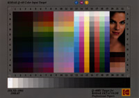
For an IT8.7/2 chart, this is the ref/it8.cht file supplied with Argyll, and  the manufacturer will will supply an individual or batch average file along with the chart containing this information, or downloadable from their web site. For instance, Kodak Q60 target reference files are here.
NOTE that the reference file for the IT8.7/2 chart supplied with Monaco EZcolor can be obtained by unzipping the .mrf file. (You may have to make a copy of the file with a .zip extension to do this.)

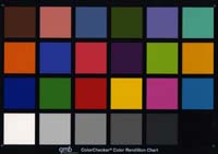
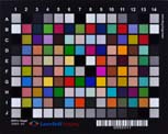
For the ColorChecker 24 patch chart, the ref/ColorChecker.cht file should be used, and there is also a ref/ColorChecker.cie file provided that is based on the manufacturers reference values for the chart. You can also create your own reference file using an instrument and chartread, making use of the chart reference file ref/ColorChecker.ti2:
   chartread -n -a ColorChecker.ti2
Note that due to the small number of patches, a profile created from such a chart is not likely to be very detailed.

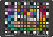
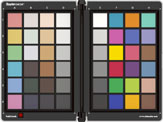
For the ColorChecker DC chart, the ref/ColorCheckerDC.cht file should be used, and there will be a ColorCheckerDC reference file supplied by X-Rite/GretagMacbeth with the chart.

The ColorChecker SG is relatively expensive, but is preferred by many people because (like the ColorChecker and ColorCheckerDC) its colors are composed of multiple different pigments, giving it reflective spectra that are more representative of the real world, unlike many other charts that are created out of combination of 3 or 4 colorants.
A limited CIE reference file is available from X-Rite here, but it is not in the usual CGATS format. To convert it to a CIE reference file useful for scanin, you will need to edit the X-Rite file using a plain text editor, first deleting everything before the line starting with "A1" and everything after "N10", then prepending this header, and appending this footer, making sure there are no blank lines inserted in the process.
If you do happen to have access to a more comprehensive instrument measurement of the ColorChecker SG, or you have measured it yourself using a color instrument,
then you may need to convert the reference information from spectral ColorCheckerSG.txt file to CIE value ColorCheckerSG.cie reference file, follow the following steps:
     txt2ti3 ColorCheckerSG.txt ColorCheckerSG
     spec2cie ColorCheckerSG.ti3 ColorCheckerSG.cie

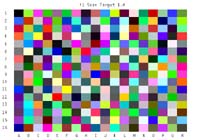
For the Eye-One Pro Scan Target 1.4 chart, the ref/i1_RGB_Scan_1.4.cht file should be used, and as there is no reference file accompanying this chart, the chart needs to be read with an instrument (usually the Eye-One Pro). This can be done using chartread,  making use of the chart reference file ref/i1_RGB_Scan_1.4.ti2:
    chartread -n -a i1_RGB_Scan_1.4
and then rename the resulting i1_RGB_Scan_1.4.ti3 file to i1_RGB_Scan_1.4.cie

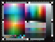
For the HutchColor HCT chart, the ref/Hutchcolor.cht file should be used, and the reference .txt file downloaded from the HutchColor website.

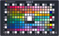
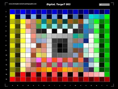
For the Christophe Métairie's Digital TargeT 003 chart with 285 patches, the ref/CMP_DT_003.cht file should be used, and the cie reference files come with the chart.

For the Christophe Métairie's Digital Target-3 chart with 570 patches, the ref/CMP_Digital_Target-3.cht file should be used, and the cie reference files come with the chart.

For the LaserSoft DCPro chart, the ref/LaserSoftDCPro.cht file should be used, and reference .txt file downloaded from the Silverfast website.

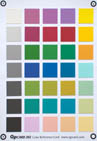
For the Datacolor SpyderCheckr, the ref/SpyderChecker.cht file should be used, and a reference ref/SpyderChecker.cie file made from measuring a sample chart is also available. Alternately you could create your own reference file by transcribing the values on the Datacolor website.

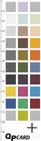
For the QPCard 201, the ref/QPcard_201.cht file should be used, and a reference ref/QPcard_201.cie file made from measuring a sample chart is also available.

For the QPCard 202, the ref/QPcard_202.cht file should be used, and a reference ref/QPcard_202.cie file made from measuring a sample chart is also available.

For any other type of chart, a chart recognition template file will need to be created (this is beyond the scope of the current documentation, although see  the .cht_format documentation).

To create the scanner .ti3 file, run the scanin tool as follows (assuming an IT8 chart is being used):

scanin -v scanner.tif It8.cht It8ref.txt

"It8ref.txt" or "It8ref.cie" is assumed to be the name of the CIE reference file supplied by the chart manufacturer. The resulting file will be named "scanner.ti3".

scanin will process 16 bit per component .tiff files, which (if the scanner is capable of creating such files),  may improve the quality of the profile.

If you have any doubts about the correctness of the chart recognition, or the subsequent profile's delta E report is unusual, then use the scanin diagnostic flags -dipn and examine the diag.tif diagnostic file, to make sure that the patches are identified and aligned correctly. If you have problems getting good automatic alignment, then consider doing a manual alignment by locating the fiducial marks on your scan, and feeding them into scanin -F parameters. The fiducial marks should be listed in a clockwise direction starting at the top left.

Creating a scanner or camera input profile

Similar to a display profile, an input profile can be either a shaper/matrix or LUT based profile. Well behaved input devices will probably give the best results with a shaper/matrix profile, and this may also be the best choice if your test chart has a small or unevenly distributed set of test patchs (ie. the IT8.7.2). If a shaper/matrix profile is a poor fit, consider using a LUT type profile.

When creating a LUT type profile, there is the choice of XYZ or L*a*b* PCS (Device independent, Profile Connection Space). Often for input devices, it is better to choose the XYZ PCS, as this may be a better fit given that input devices are usually close to being linearly additive in behaviour.

If the purpose of the input profile is to use it as a substitute for a colorimeter, then the -u flag should be used to avoid clipping values above the white point. Unless the shaper/matrix type profile is a very good fit, it is probably advisable to use a LUT type profile in this situation.

To create a matrix/shaper profile, the following suffices:

colprof -v -D"Scanner A" -qm -as scanner

For an XYZ PCS LUT based profile then the following would be used:

colprof -v -D"Scanner A" -qm -ax scanner

For the purposes of a poor mans colorimeter, the following would generally be used:

colprof -v -D"Scanner A" -qm -ax -u scanner

Make sure you check the delta E report at the end of the profile creation, to see if the profile is behaving reasonably.


If profiling a camera in RAW mode, then there may be some advantage in creating a pure matrix only profile, in which it is assumed that the camera response is completely linear. This may reduce extrapolation artefacts. If setting the white point will be done in some application, then it may also be an advantage to use the -u flag and avoid setting the white point to that of the profile chart:

colprof -v -D"Camera" -qm -am -u scanner


Profiling Printers

The overall process is to create a set of device measurement target values, print them out, measure them, and then create an ICC profile from the measurements. If the printer is an RGB based printer, then the process is only slightly more complicated than profiling a display. If the printer is CMYK based, then some additional parameters are required to set the total ink limit (TAC) and  black generation curve.

Creating a print profile test chart

The first step in profiling any output device, is to create a set of device colorspace test values. The important parameters needed are:
Most printers running through simple drivers will appear as if they are RGB devices. In fact there is no such thing as a real RGB printer, since printers use white media and the colorant must subtract from the light reflected on it to create color, but the printer itself turns the incoming RGB into the native print colorspace, so for this reason we will tell targen to use the "Print RGB" colorspace, so that it knows that it's really a subtractive media. Other drivers will drive a printer more directly, and will expect a CMYK profile. [Currently Argyll is not capable of creating an ICC profile for devices with more colorants than CMYK. When this capability is introduced, it will by creating an additional separation profile which then allows the printer to be treated as a CMY or CMYK printer.] One way of telling what sort of profile is expected for your device is to examine an existing profile for that device using iccdump.

The number of test patches will depend somewhat on what quality profile you want to make, how well behaved the printer is, as well as the effort needed to read the number of test values. Generally it is convenient to fill a certain paper size with the maximum number of test values that will fit.

At a minimum, for an "RGB" device, a few hundred values are needed (400-1000). For high quality CMYK profiles, 1000-3000 is not an unreasonable number of patches.

To assist the determination of test patch values, it can help to have a rough idea of how the device behaves, so that the device test point locations can be pre-conditioned. This could be in the form of an ICC profile of a similar device, or a lower quality, or previous profile for that particular device. If one were going to make a very high quality Lut based profile, then it might be worthwhile to make up a smaller, preliminary shaper/matrix profile using a few hundred test points, before embarking on testing the device with several thousand.

The documentation for the targen tool lists a table of paper sizes and number of  patches for typical situations.

For a CMYK device, a total ink limit usually needs to be specified. Sometimes a device will have a maximum total ink limit set by its manufacturer or operator, and some CMYK systems (such as chemical proofing systems) don't have any limit. Typical printing devices such as Xerographic printers, inkjet printers and printing presses will have a limit. The exact procedure for determining an ink limit is outside the scope of this document, but one way of going about this might be to generate some small (say a few hundred patches) with targen & pritntarg with different total ink limits, and printing them out, making the ink limit as large as possible without striking problems that are caused by too much ink.

Generally one wants to use the maximum possible amount of ink to maximize the gamut available on the device. For most CMYK devices, an ink limit between 200 and 400 is usual, but and ink limit of 250% or over is generally desirable for reasonably dense blacks and dark saturated colors. And ink limit of less than 200% will begin to compromise the fully saturated gamut, as secondary colors (ie combinations of any two primary colorants) will not be able to reach full strength.

Once an ink limit is used in printing the characterization test chart for a device, it becomes a critical parameter in knowing what the characterized gamut of the device is. If after printing the test chart, a greater ink limit were to be used, the the software would effectively be extrapolating the device behaviour at total ink levels beyond that used in the test chart, leading to inaccuracies.

Generally in Argyll, the ink limit is established when creating the test chart values, and then carried through the profile making process automatically. Once the profile has been made however, the ink limit is no longer recorded, and you, the user, will have to keep track of it if the ICC profile is used in any program than needs to know the usable gamut of the device.


Lets consider two devices in our examples, "PrinterA" which is an "RGB" device, and "PrinterB" which is CMYK, and has a target ink limit of 250%.

The simplest approach is to make a set of test values that is independent of the characteristics of the particular device:

targen -v  -d2 -f1053 PrinterA

targen -v  -d4 -l260 -f1053 PrinterB

The number of patches chosen here happens to be right for an A4 paper size being read using a Spectroscan instrument. See the table in  the targen documentation for some other suggested numbers.

If there is a preliminary or previous profile called "OldPrinterA" available, and we want to try creating a "pre-conditioned" set of test values that will more efficiently sample the device response, then the following would achieve this:

targen -v  -d2 -f1053 -c OldPrinterA PrinterA

targen -v  -d4 -l260 -f1053 -c OldPrinterB PrinterB


The output of targen will be the file PrinterA.ti1 and PrinterB.ti1 respectively, containing the device space test values, as well as expected CIE values used for chart recognition purposes.

Printing a print profile test chart

The next step is turn the test values in to a PostScript or TIFF raster test file that can printed on the device. The basic information that needs to be supplied is the type of instrument that will be used to read the patches, as well as the paper size it is to be formatted for.

For an X-Rite DTP41, the following would be typical:

printtarg -v -i41 -pA4 PrinterA
 
For a Gretag Eye-One Pro, the following would be typical:

printtarg -v -ii1 -pA4 PrinterA

For using with a scanner as a colorimeter, the Gretag Spectroscan layout is suitable, but the -s flag should be used so as to generate a layout suitable for scan recognition, as well as generating the scan recognition template files. (You probably want to use less patches with targen, when using the printtarg -s flag, e.g. 1026 patches for an A4R page, etc.) The following would be typical:

printtarg -v -s -iSS -pA4R PrinterA

printtarg
reads the PrinterA.ti1 file, creates a PrinterA.ti2 file containing the layout information as well as the device values and expected CIE values, as well as a PrinterA.ps file containing the test chart. If the -s flag is used, one or more PrinterA.cht files is created to allow the scanin program to recognize the chart.

To create TIFF raster files rather than PostScript, use the -t flag.

GSview is a good program to use to check what the PostScript file will look like, without actually printing it out. You could also use Photoshop or ImageMagick for this purpose.

The last step is to print the chart out.

Using a suitable PostScript or raster file printing program, downloader, print the chart. If you are not using a TIFF test chart, and you do not have a PostScript capable printer, then an interpreter like GhostScript or even Photoshop could be used to rasterize the file into something that can be printed. Note that it is important that the PostScript interpreter or TIFF printing application and printer configuration is setup for a device profiling run, and that any sort of color conversion of color correction be turned off so that the device values in the PostScript or TIFF file are sent directly to the device. If the device has a calibration system, then it would be usual to have setup and calibrated the device before starting the profiling run, and to apply calibration to the chart values. If Photoshop was to be used, then either the chart needs to be a single page, or separate .eps or .tiff files for each page should be used, so that they can be converted and printed one at a time (see the -e and -t flags).

Reading a print test chart using an instrument

Once the test chart has been printed, the color of the patches needs to be read using a suitable instrument.

Several different instruments are currently supported, some that need to be used patch by patch, some read a strip at a time, and some read a sheet at a time. See instruments for a current list.

The instrument needs to be connected to your computer before running the chartread command. Both serial port and USB connected Instruments are supported. A serial port to USB adapter might have to be used if your computer doesn't have any serial ports, and you have a serial interface connected instrument.

If you run chartread so as to print out its usage message (ie. by using a -? or -- flags), then it will list any identified serial ports or USB connected instruments, and their corresponding number for the -c option. By default, chartread will try to connect to the first available USB instrument, or an instrument on the first serial port.

The only arguments required is to specify the basename of the .ti2 file. If a non-default serial port is to be used, then the -c option would also be specified.

 e.g. for a Spectroscan on the second port:

chartread -c2 PrinterA

For a DTP41 to the default serial port:

chartread PrinterA

chartread will interactively prompt you through the process of reading each sheet or strip. See chartread for more details on the responses for each type of instrument. Continue with Creating a printer profile.

Reading a print test chart using a scanner or camera


Argyll supports using a scanner or even a camera as a substitute for a colorimeter. While a scanner or camera is no replacement for a color measurement instrument, it may give acceptable results in some situations, and may give better results than a generic profile for a printing device.

The main limitation of the scanner-as-colorimeter approach are:

* The scanner dynamic range and/or precision may not match the printers or what is required for a good profile.
* The spectral interaction of the scanner test chart and printer test chart with the scanner spectral response can cause color errors.
* Spectral differences caused by different black amounts in the print test chart can cause color errors.
* The scanner reference chart gamut may be much smaller than the printers gamut, making the scanner profile too inaccurate to be useful.

As well as some of the above, a camera may not be suitable if it automatically adjusts exposure or white point when taking a picture, and this behavior cannot be disabled.

The end result is often a profile that has a noticeable color cast, compared to a profile created using a colorimeter or spectrometer.


It is assumed that you have created a scanner or camera profile following the procedure outline above. For best possible results it is advisable to both profile the scanner or camera, and use it in scanning the printed test chart, in as "raw" mode as possible (i.e. using 16 bits per component images, if the scanner or camera is capable of doing so; not setting white or black points, using a fixed exposure etc.). It is generally advisable to create a LUT type input profile, and use the -u flag to avoid clipping scanned value whiter than the input calibration chart.

Scan or photograph your printer chart (or charts) on the scanner or camera previously profiled. The scanner or camera must be configured and used exactly the same as it was when it was profiled.

I will assume the resulting scan/photo input file is called PrinterB.tif (or PrinterB1.tif, PrinterB2.tif etc. in the case of multiple charts). As with profiling the scanner or camera, the raster file need only be roughly cropped so as to contain the test chart.

The scanner recognition files created when printtarg was run is assumed to be called PrinterB.cht. Using the scanner profile created previously (assumed to be called scanner.icm), the printer test chart scan patches are converted to CIE values using the scanin tool:

scanin -v -c PrinterB.tif PrinterB.cht scanner.icm PrinterB

If there were multiple test chart pages, the results would be accumulated page by page using the -ca option, ie., if there were 3 pages:

scanin -v -c PrinterB1.tif PrinterB1.cht scanner.icm PrinterB
scanin -v -ca PrinterB2.tif PrinterB2.cht scanner.icm PrinterB
scanin -v -ca PrinterB3.tif PrinterB3.cht scanner.icm PrinterB

Now that the PrinterB.ti3 data has been obtained, the profile continue in the next section with Creating a printer profile.

If you have any doubts about the correctness of the chart recognition, or the subsequent profile's delta E report is unusual, then use the scanin diagnostic flags -dipn and examine the diag.tif diagnostic file.

Creating a printer profile

Creating an RGB based printing profile is very similar to creating a display device profile. For a CMYK printer, some additional information is needed to set the black generation.

Where the resulting profile will be used conventionally (ie. using collink -s, or cctiff or most other "dumb" CMMs) it is important to specify that gamut mapping should be computed for the output (B2A) perceptual and saturation tables. This is done by specifying a device profile as the parameter to the colprof -S flag. When you intend to create a "general use" profile, it can be a good technique to specify the source gamut as the opposite type of profile to that being created, i.e. if a printer profile is being created, specify a display profile (e.g. sRGB) as the source gamut. If a display profile is being created, then specify a printer profile as the source (e.g. Figra, SWOP etc.).  When linking to the profile you have created this way as the output profile, then use perceptual intent if the source is the opposite type, and relative colorimetric if it is the same type.

"Opposite type of profile" refers to the native gamut of the device, and what its fundamental nature is, additive or subtractive. An emissive display will have additive primaries (R, G & B), while a reflective print, will have subtractive primaries (C, M, Y & possibly others), irrespective of what colorspace the printer is driven in (a printer might present an RGB interface, but internally this will be converted to CMY, and it will have a CMY type of gamut).  Because of the complimentary nature of additive and subtractive device primary colorants, these types of devices have the most different gamuts, and hence need the most gamut mapping to convert from one colorspace to the other.

If you are creating a profile for a specific purpose, intending to link it to a specific input profile, then you will get the best results by specifying that source profile as the source gamut.

If a profile is only going to be used as an input profile, or is going to be used with a "smart" CMM (e.g. collink -g or -G), then it can save considerable processing time and space if the -b flag is used, and the -S flag not used.

For an RGB printer intended to print RGB originals, the following might be a typical profile usage:

colprof -v -D"Printer A" -qm -S sRGB.icm -cmt -dpp PrinterA

or if you intent to print from Fogra, SWOP or other standard CMYK style originals:

colprof -v -D"Printer A" -qm -S fogra39l.icm -cmt -dpp PrinterA

If you know what colorspace your originals are in, use that as the argument to -S.

Choosing a black generation curve (and other CMYK printer options)

For a CMYK printer, it would be normal to specify the type of black generation, either as something simple, or as a specific curve. The documentation  in colprof for the details of the options.

Note
that making a good choice of black generation curve can affect things such as: how robust neutrals are given printer drift or changes in viewing lighting, how visible screening is, and how smooth looking the B2A conversion is.

For instance, maximizing the level of K will mean that the neutral colors are composed of greater amounts of Black ink, and black ink retains its neutral appearance irrespective of printer behavior or the spectrum of the illuminant used to view the print. On the other hand, output which is dominantly from one of the color channels will tend to emphasize the screening pattern and any unevenness (banding etc.) of that channel, and the black channel in particular has the highest visibility. So in practice, some balance between the levels of the four channels is probably best, with more K if the screening is fine and a robust neutral balance is important, or less K if the screening is more visible and neutral balance is less critical. The levels of K at the edges of the gamut of the device will be fixed by the nature of the ink combinations that maximize the gamut (ie. typically zero ink for light chromatic colors, some combination for dark colors, and a high level of black for very dark near neutrals), and it is also usually important to set a curve that smoothly transitions to the K values at the gamut edges. Dramatic changes in K imply equally dramatic changes in CMY, and these abrupt transitions will reveal the limited precision and detail that can be captured in a lookup table based profile, often resulting in a "bumpy" looking output.

If you want to experiment with the various black generation parameters, then it might be a good idea to create a preliminary profile (using -ql -b -no, -ni and no -S), and then used xicclu to explore the effect of the parameters.

For instance, say we have our CMYK .ti3 file PrinterB.ti3. First we make a preliminary profile called PrinterBt:

copy PrinterB.ti3 PrinterBt.ti3      (Use "cp" on Linux or OSX of course.)
colprof -v -qm -b -cmt -dpp PrinterBt

Then see what the minimum black level down the neutral axis can be. Note that we need to also set any ink limits we've decided on as well (coloprof defaulting to 10% less than the value recorded in the .ti3 file). In this example the test chart has a 300% total ink limit, and we've decided to use 290%:

xicclu -g -kz -l290 -fif -ir PrinterBt.icm

Which might be a graph something like this:

Graph of CMYK neutral axis with minimum K

Note  how the minimum black is zero up to 93% of the white->black L* curve, and then jumps up to 87%. This is because we've reached the total ink limit, and K then has to be substituted for CMY, to keep the total under the total ink limit.

Then let's see what the maximum black level down the neutral axis can be:

xicclu -g -kx -l290 -fif -ir PrinterBt.icm

Which might be a graph something like this:

Graph of CMYK neutral axis with maximum K

Note how the CMY values are fairly low up to 93% of the white->black L* curve (the low levels of CMY are helping set the neutral color), and then they jump up. This is because we've reach the point where black on it's own, isn't as dark as the color that can be achieved using CMY and K. Because the K has a dominant effect on the hue of the black, the levels of CMY are often fairly volatile in this region.

Any K curve we specify must lie between the black curves of the above two graphs.

Let's say we'd like to chose a moderate black curve, one that aims for about equal levels of CMY and K. We should also aim for it to be fairly smooth, since this will minimize visual artefacts caused by the limited fidelity that profile LUT tables are able to represent inside the profile.

-k parameters


For minimum discontinuities we should aim for the curve to finish at the point it has to reach to satisfy the total ink limit at 87% curve and 93% black. For a first try we can simply set a straight line to that point:

xicclu -g -kp 0 0 .93 .87 1.0 -l290 -fif -ir PrinterBt.icm

Graph of CMYK neutral axis with kp 0 0 1.0 1.0 1.0 -l290

The black "curve" hits the 93%/87% mark well, but is a bit too far above CMY, so we'll try making the black curve concave:

xicclu -g -kp 0 0 .93 .87 0.65 -l290 -fif -ir PrinterBt.icm

Graph of CMYK neutral axis with -kp 0 .05 1 .9 1 -l290

This looks just about perfect, so the the curve parameters can now be used to generate our real profile:

colprof -v -D"Printer B" -qm -kp 0 0 .93 .87 0.65 -S sRGB.icm -cmt -dpp PrinterB

and the resulting B2A table black curve can be checked using xicclu:

xicclu -g -fb -ir PrinterB.icm

sadsadas


Examples of other inkings:

A smoothed zero black inking:

xicclu -g -kp 0 .7 .93 .87 1.0 -l290 -fif -ir PrinterBt.icm

sadsadas

A low black inking:

xicclu -g -kp 0 0 .93 .87 0.15 -l290 -fif -ir PrinterBt.icm

sadsadas


A high black inking:

xicclu -g -kp 0 0 .93 .87 1.2 -l290 -fif -ir PrinterBt.icm

sadsadas

Overriding the ink limit

Normally the total ink limit will be read from the PrinterB.ti3 file, and will be set at a level 10% lower than the number used in creating the test chart values using targen -l. If you want to override this with a lower limit, then use the -l flag.

colprof -v -D"Printer B" -qm -S sRGB.icm -cmt -dpp -kr -l290 PrinterB

Make sure you check the delta E report at the end of the profile creation, to see if the profile is behaving reasonably.

One way of checking that your ink limit is not too high, is to use "xicc -fif -ia" to check, by setting different ink limits using the -l option, feeding Lab = 0 0 0 into it, and checking the resulting  black point. Starting with the ink limit used with targen for the test chart, reduce it until the black point starts to be affected. If it is immediately affected by any reduction in the ink limit, then the black point may be improved by increasing the ink limit used to generate the test chart and then re-print and re-measuring it, assuming other aspects such as wetness, smudging, spreading or drying time are not an issue.


Calibrating Printers

Profiling creates a description of how a device behaves, while calibration on the other hand is intended to change how a device behaves. Argyll has the ability to create per-channel device space calibration curves for print devices, that can then be used to improve the behavior of of the device, making a subsequent profile fit the device more easily and also allow day to day correction of device drift without resorting to a full re-profile.

NOTE: Because calibration adds yet another layer to the way color is processed, it is recommended that it not be attempted until the normal profiling workflow is established, understood and verified.

Calibrated print workflows

There are two main workflows that printer calibration curves can be applied to:

Workflow with native calibration capability:

Firstly the printer itself may have the capability of using per channel calibration curves. In this situation, the calibration process will be largely independent of profiling. Firstly the printer is configured to have both its color management and calibration disabled (the latter perhaps achieved by loading linear calibration curves), and a print calibration test chart that consists of per channel color wedges is printed. The calibration chart is read and the resulting .ti3 file converted into calibration curves by processing it using printcal. The calibration is then installed into the printer. Subsequent profiling will be performed on the calibrated printer (ie. the profile test chart will have the calibration curves applied to it by the printer, and the resulting ICC profile will represent the behavior of the calibrated printer.)

Workflow without native calibration capability:

The second workflow is one in which the printer has no calibration capability itself. In this situation, the calibration process will have to be applied using the ICC color management tools, so careful coordination with profiling is needed. Firstly the printer is configured to have its color management disabled, and a print calibration test chart that consists of per channel color wedges is printed. The calibration chart is converted into calibration curves by reading it and then processing the resultant .ti3 using printcal,. During the subsequent profiling, the calibration curves will need to be applied to the profile test chart in the process of using printtarg. Once the the profile has been created, then in subsequent printing the calibration curves will need to be applied to an image being printed either explicitly when using cctiff to apply color profiles and calibration, OR by creating a version of the profile that has had the calibration curves incorporated into it using the applycal tool. The latter is useful when some CMM (color management module) other than cctiff is being used.

Once calibration aim targets for a particular device and mode (screening, paper etc.) have been established, then the printer can be re-calibrated at any time to bring its per channel behavior back into line if it drifts, and the new calibration curves can be installed into the printer, or re-incorporated into the profile.  

Creating a print calibration test chart

The first step is to create a print calibration test chart. Since calibration only creates per-channel curves, only single channel step wedges are required for the chart. The main choice is the number of steps in each wedge. For simple fast calibrations perhaps as few as 20 steps per channel may be enough, but for a better quality of calibration something like 50 or more steps would be a better choice.

Let's consider two devices in our examples, "PrinterA" which is an "RGB" printer device, and "PrinterB" which is CMYK. In fact there is no such thing as a real RGB printer, since printers use white media and the colorant must subtract from the light reflected on it to create color, but the printer itself turns the incoming RGB into the native print colorspace, so for this reason we are careful to tell targen to use the "Print RGB" colorspace, so that it knows to create step wedges from media white to full colorant values.

For instance, to create a 50 steps per channel calibration test chart for our RGB and CMYK devices, the following would be sufficient:

targen -v  -d2 -s50 -e3 -f0 PrinterA_c

targen -v  -d4 -s50 -e4 -f0 PrinterB_c

For an outline of how to then print and read the resulting test chart, see  Printing a print profile test chart, and Reading a print test chart using an instrument. Note that the printer must be in an un-profiled and un-calibrated mode when doing this print. Having done this, there will be a PrinterA.ti3 or PrinterB.ti3 file containing the step wedge calibration chart readings.

NOTE that if you are calibrating a raw printer driver, and there is considerable dot gain, then you may want to use the -p parameter to adjust the test chart point distribution to spread them more evenly in perceptual space, giving more accurate control over the calibration. Typically this will be a value greater than one for a device that has dot gain, e.g. values of 1.5, 2.0 or 2.5 might be good places to start. You can do a preliminary calibration and use the verbose output of printcal to recommend a suitable value for -p.

Creating a printer calibration

The printcal tool turns a calibration chart .ti3 file into a .cal file. It has three main operating modes:- Initial calibration, Re-Calibration, and Verification. (A fourth mode, "Imitation" is very like Initial Calibration, but is used for establishing a calibration target that a similar printer can attempt to imitate.)

The distinction between Initial Calibration and Re-Calibration is that in the initial calibration we establish the "aim points" or response we want out of the printer after calibration. There are three basic parameters to set this for each channel: Maximum level, minimum level, and curve shape.

By default the maximum level will be set using a heuristic which attempts to pick the point when there is diminishing returns for applying more colorant. This can be overridden using the -x# percent option, where # represents the choice of channel this will be applied to. The parameter is the percentage of device maximum.

The minimum level defaults to 0, but can be overridden using the -n# deltaE option. A minimum of 0 means that zero colorant will correspond to the natural media color, but it may be desirable to set a non-pure media color using calibration for the purposes of emulating some other media. The parameter is in Delta E units.

The curve shape defaults to being perceptually uniform, which means that even steps of calibrated device value result in perceptually even color steps. In some situations it may be desirable to alter this curve (for instance when non color managed output needs to be sent to the calibrated printer), and a simple curve shape target can be set using the -t# percent parameter. This affects the output value at 50% input value, and represents the percentage of perceptual output. By default it is 50% perceptual output for 50% device input.

Once a device has been calibrated, it can be re-calibrated to the same aim target.

Verification uses a calibration test chart printed through the calibration, and compares the achieved response to the aim target.

The simplest possible way of creating the PrinterA.cal file is:

  printcal -i PrinterA_c

For more detailed information, you can add the -v and -p flags:

  printcal -v -p -i PrinterB_c

(You will need to select the plot window and hit a key to advance past each plot).

For re-calibration, the name of the previous calibration file will need to be supplied, and a new calibration
file will be created:

  printcal -v -p -r PrinterB_c_old PrinterB_c_new

Various aim points are normally set automatically by printcal, but these can be overridden using the -x, -n and -t options. e.g. say we wanted to set the maximum ink for Cyan to 80% and Black to 95%, we might use:

  printcal -v -p -i -xc 80 -xk 95 PrinterB_c

Using a printer calibration

The resulting calibration curves can be used with the following other Argyll tools:

    printtarg     To apply calibration to a profile test chart, and/or to have it included in .ti3 file.
    cctiff         To apply color management and calibration to an image file.
    applycal     To incorporate calibration into an ICC profile.
    chartread   To override the calibration assumed when reading a profile chart.


In a workflow with native calibration capability, the calibration curves would be used with printarg during subsequent profiling so that any ink limit calculations will reflect final device values, while not otherwise using the calibration within the ICC workflow:

    printtarg -v -ii1 -pA4 -I PrinterA_c.cal PrinterA

This will cause the .ti2 and resulting .ti3 and ICC profiles to contain the calibration curves, allowing all the tools to be able to compute final device value ink limits. The calibration curves must also of course be installed into the printer. The means to do this is currently outside the scope of Argyll (ie. either the print system needs to be able to understand Argyll CAL format files, or some tool will be needed to convert Argyll CAL files into the printer calibration format).


In a workflow without native calibration capability, the calibration curves would be used with printarg to apply the calibration to the test patch samples during subsequent profiling, as well as embedding it in the resulting .ti3 to allow all the tools to be able to compute final device value ink limits:

    printtarg -v -ii1 -pA4 -K PrinterA_c.cal PrinterA

To apply calibration to an ICC profile, so that a calibration unaware CMM can be used:

    applycal PrinterA.cal PrinterA.icm PrinterA_cal.icm

To apply color management and calibration to a raster image:

    cctiff Source2Destination.icm PrinterA_c.cal infile.tif outfile.tif
or
    cctiff Source2Destination.icm PrinterA_c.cal infile.jpg outfile.jpg


Another useful tool is synthcal, that allows creating linear or synthetic calibration files for disabling calibration or testing.
Similarly, fakeread also supports applying calibration curves and embedding them in the resulting .ti3 file

How profile ink limits are handled when calibration is being used.

Even though the profiling process is carried out on top of the linearized device, and the profiling is generally unaware of the underlying non-linearized device values, an exception is made in the calculation of ink limits during profiling. This is made possible by including the calibration curves in the profile charts .ti2 and subsequent .ti3 file and resulting ICC profile 'targ' text tag, by way of the printtarg -I or -K options. This is done on the assumption that the physical quantity of ink is what's important in setting the ink limit, and that the underlying non-linearized device values represent such a physical quantity.


Linking Profiles

Two device profiles can be linked together to create a device link profile, than encapsulates a particular device to device transform. Often this step is not necessary, as many systems and tools will link two device profiles "on the fly", but creating a device link profile gives you the option of using "smart CMM" techniques, such as true gamut mapping, improved inverse transform accuracy, tailored black generation and ink limiting.

The overall process is to link the input space and output space profiles using collink, creating a device to device link profile. The device to device link profile can then be used by cctiff (or other ICC device profile capable tools), to color correct a raster files.

Three examples will be given here, showing the three different modes than collink supports.

In simple mode, the two profiles are linked together in a similar fashion to other CMMs simply using the forward and backwards color transforms defined by the profiles. Any gamut mapping is determined by the content of the tables within the two profiles, together with the particular intent chosen. Typically the same intent will be used for both the source and destination profile:

collink -v -qm -s -ip -op SouceProfile.icm DestinationProfile.icm Source2Destination.icm


In gamut mapping mode, the pre-computed intent mappings inside the profiles are not used, but instead the gamut mapping between source and destination is tailored to the specific gamuts of the two profiles, and the intent parameter supplied to collink. Additionally, source and destination viewing conditions should be provided, to allow the color appearance space conversion to work as intended. The colorimetric B2A table in the destination profile is used, and this will determine any black generation and ink limiting:

collink -v -qm -g -ip -cmt -dpp MonitorSouceProfile.icm DestinationProfile.icm Source2Destination.icm


In inverse output table gamut mapping mode, the pre-computed intent mappings inside the profiles are not used, but instead the gamut mapping between source and destination is tailored to the specific gamuts of the two profiles, and the intent parameter supplied to collink. In addition, the B2A table is not used in the destination profile, but the A2B table is instead inverted, leading to improved transform accuracy, and in CMYK devices, allowing the ink limiting and black generation parameters to be set:

For a CLUT table based RGB printer destination profile, the following would be appropriate:

collink -v -qm -G -ip -cmt -dpp MonitorSouceProfile.icm RGBDestinationProfile.icm Source2Destination.icm

For a CMYK profile, the total ink limit needs to be specified (a typical value being 10% less than the value used in creating the device test chart), and the type of black generation also needs to be specified:

collink -v -qm -G -ip -cmt -dpp -l250 -kr MonitorSouceProfile.icm CMYKDestinationProfile.icm Source2Destination.icm

Note that you should set the source (-c) and destination (-d) viewing conditions for the type of device the profile represents, and the conditions under which it will be viewed.

Soft Proofing Link

Often it is desirable to get an idea what a particular devices output will look like using a different device. Typically this might be trying to evaluate print output using a display. Often it is sufficient to use an absolute or relative colorimetric transform from the print device space to the display space, but while these provide a colorimetric preview of the result, they do not take into account the subjective appearance differences due to the different device conditions. It can therefore be useful to create a soft proof appearance transform using collink:

collink -v -qm -G -ila -cpp -dmt -t250 CMYKDestinationProfile.icm MonitorProfile.icm SoftProof.icm

We use the Luminance matched appearance intent, to preserve the subjective apperance of the target device, which takes into account the viewing conditions and assumes adaptation to the differences in the luminence range, but otherwise not attempting to compress or change the gamut.
 

Transforming colorspaces of raster files

Although a device profile or device link profile may be useful with other programs and systems, Argyll provides the tool cctiff for directly applying a device to device transform to a TIFF or JPEG raster file. The cctiff tool is capable of linking an arbitrary sequence of device profiles, device links, abstract profiles and calibration curves. Each device profile can be preceded by the -i option to indicate the intent that should be used. Both 8 and 16 bit per component files can be handled, and up to 8 color channels. The color transform is optimized to perform the overall transformation rapidly.

If a device link is to be used, the following is a typical example:

cctiff Source2Destination.icm infile.tif outfile.tif
or
cctiff Source2Destination.icm infile.jpg outfile.jpg


If a source and destination profile are to be used, the following would be a typical example:

cctiff  -ip SourceProfile.icm -ip DestinationProfile.icm infile.tif outfile.tif
or
cctiff  -ip SourceProfile.icm -ip DestinationProfile.icm infile.jpg outfile.jpg